Hopfield Network Python implementation

What is a Hopfield Network?

Hopfield networks, introduced by physicist John Joseph Hopfield in 1982, offer a fascinating perspective on the workings of associative memory — a mechanism that allows us to recall information based on its content, much like when a scent evokes a childhood memory. Hopfield, who won the Nobel Prize in Physics in 2024 alongside Geoffrey Hinton for their pioneering role in developing neural networks, designed a model that captures the essence of this process within an artificial system.

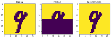
A Hopfield network can perform two primary tasks: pattern recognition and error correction. It can store a set of patterns (binary vectors) in its memory, and when a new input is presented, the network will try to recall the closest stored pattern, even if the input is incomplete or noisy. This process is known as auto-association, where the network can reconstruct a full pattern from a partial one. For example, if the net has learned to store images, it can recognize an image even if parts are missing or distorted, retrieving the correct version from memory.

How it works?

A Hopfield network is composed of the following main components:

Neurons (Node)
- Each neuron in the network represents a binary unit that can have a state of either $+1$ (active) or $-1$ (inactive). Neurons are both input and output units, meaning they receive inputs and produce outputs. They are fully connected, which means every neuron is connected to every other neuron.
- The current configuration of the network can be represented as a state vector $\mathbf{s} = [s_1, s_2, \ldots, s_N]$ , where N is the total number of neurons. Each element s_i indicates the state of neuron i . The network’s goal is to update this state vector until it reaches a stable, low-energy state.
Weights ( $w_{ij}$ $w_{ij}$ )
- The connections between neurons are defined by weights $w_{ij},$ which determine the strength and nature (excitatory or inhibitory) of the connections. The weights are symmetric ( $w_{ij} = w_{ji}$ ), ensuring that the influence between two neurons is mutual. Weights are learned during the training phase, where patterns are stored in the network.
- The weight matrix is calculated via Hebb's law of association (the outer product of the image vector): $w_{ij} = \sum_{\mu=1}^{p} s_i^\mu s_j^\mu$
  
  where $s_i^\mu$ and $s_j^\mu$ are the elements of the binary vector representing the stored pattern $\mu$ .
Update Rule ( auto-association )
- The network relies on an update rule to change the states of neurons. This can be done synchronously (all neurons update at once) or asynchronously (one neuron at a time). The rule is:
  
  $s_i = \text{sign} \left( \sum_{j} w_{ij} s_j \right)$

Python implementation

Let’s write some code for demonstrates how a Hopfield network can be used to store and reconstruct multiple images.

Import libraries

1 2 3import numpy as np #for numerical operations import matplotlib.pyplot as plt #for displaying images(array) from PIL import Image #for image processing
Image processing functions

1 2 3 4 5 6 7 8 9 10 11 12 13 14 15 16 17 18 19 20 21def load_img(path, side): #Load and process images into a binary array, where pixels are represented as 1 or -1 img = Image.open(path) img = img.resize((side, side)) img = img.convert('1') img = 2 * np.array(img, int) -1 return img.flatten() def show_array(img_array): #Visualize images(array) side = int(np.sqrt(img_array.shape[0])) img_array = img_array.reshape((side, side)) plt.figure(figsize=(3, 3)) plt.imshow(img_array) plt.axis('off') plt.show() def modify_img(n, img): #Introduce noise or modifications to an image, for testing the network’s ability to reconstruct it #make 1/2% of image negative for i in range(n): if i > n/2-1: img[i] = -1 return img
Hopfield net equations

1 2 3 4 5 6 7 8 9 10 11 12 13 14 15 16 17 18 19 20#weigths matrix def calculate_w(img): #Create a weight matrix using the Hebbian learning rule based on the outer product of the image vector. ''' w = np.zeros((n,n)) for i in range(n): for j in range(n): if i!=j: w[i,j]=img[i]*img[j] ''' return np.outer(img, img) #reconstruct image def reconstructed_image(n, w, state): #Use the weight matrix to reconstruct an image from a modified or noisy version for i in range(n): sum = 0 for j in range(n): sum += w[i,j]*state[j] state[i] = 1 if sum>0 else -1 return state #return np.dot(w, state)

Here is an example of a Hopfield network that memorizes 5 different patterns and reconstructs them from a modified pattern:

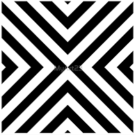
Pattern 1

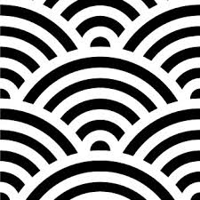
Pattern 2

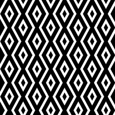
Pattern 3

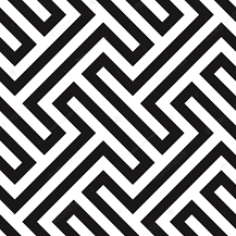
Pattern 4

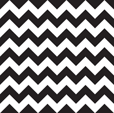
Pattern 5

Now let's run the code and analyze the results:

#multile patterns memory
side = 50
n = side * side #number of neurons(pixels)

#memory images
imgs=[]
for i in range(1,6): #memorize images from 1 to x-1
  imgs.append(load_img(f'p{i}.jpeg', side))

print('memorized images:')
show_multiple_arraysi(imgs)

#weights matrix
w = np.zeros((n,n))
for p in range(len(imgs)):
  w+=calculate_w(imgs[p])

#set inital state
state = modify_img(n, load_img('p2.jpeg', side)) #modified image
#state = np.random.choice([-1,1], size=n) #random pixels
print('init state:')
show_array(state)

#reconstruct image
state = reconstructed_image(n, w, state)
print('reconstructed image:')
show_array(state)

Output:

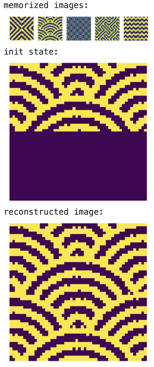
Screenshot 2024-10-18 alle 13.55.28.png

As we can see from the output, the Hopfield network successfully reconstructed the original image (p2.jpeg) from the modified input. This demonstrates the network's ability to recover stored patterns even when presented with noisy or incomplete data. The reconstructed image closely resembles the original, showcasing the power of associative memory.

Conclusion

Hopfield networks are a powerful model for associative memory, capable of storing and retrieving binary patterns. In the example, we demonstrated how the network can memorize multiple patterns and successfully reconstruct one of them, even when the input is noisy or partially altered. This ability to recall original patterns from distorted inputs highlights the network’s use in tasks like error correction and pattern recognition.

However, Hopfield networks also have limitations. One key limitation is their storage capacity. The network can store up to approximately 0.15 × N patterns reliably, where N is the number of neurons. If more patterns are stored, the network may struggle to distinguish between them, leading to incorrect reconstructions or “spurious states” that don’t correspond to any of the stored patterns. Despite this, Hopfield networks laid foundational principles for later neural network models and remain a fundamental concept in the field of artificial intelligence and cognitive science.